Code
%load_ext autoreload
%autoreload 2
import torch
from notebook_setup import device
torch.manual_seed(0)
import warnings
# Suppress specific warnings
warnings.filterwarnings("ignore", message=".*IProgress not found.*")This is a Jupyter notebook that will guide you through how to use our codebase to perform OOD detection. For simplicity, we consider OOD detection between the two greuscale image datasets: FMNIST and MNIST, where once we train a model on FMNIST and try to predict MNIST points as out-of-distribution, and another time train a model on MNIST and try to predict FMNIST as out-of-distribution. Once you have gone through these steps, you can easily extend it to other dataset pairs, or even introduce your own datasets to perform OOD detection.
Before we start, it is recommended to run the following script that downloads all the necessary resources that we will use in this notebool such as model checkpoints that are already trained on MNIST and FMNIST datasets, alongside some report files that we have already run on these models.
python scripts/download_resources.pyThe approach we follow here is that we will use some of the python scripts in the repository that output useful logs onto mlflow, such as the likelihood of different datapoints on different models. Then, we will use these logs and artifacts to visualize the results here. Make sure you run your scripts on the root of the repository and that you have followed the setup instructions to have mlflow running. Before we proceed, please run the following cell to import the necessary libraries and functions.
%load_ext autoreload
%autoreload 2
import torch
from notebook_setup import device
torch.manual_seed(0)
import warnings
# Suppress specific warnings
warnings.filterwarnings("ignore", message=".*IProgress not found.*")Here, we will work with diffusion and flow models that have been trained on MNIST and FMNIST datasets. Run the following bash commands to get 4 different mlflow logs for each model. If you have setup the repository correctly, this will produce an artifact file that contains a <artifact_dir>/samples_grid/xxx.png that contains relevant samples produces by these models.
# diffusion trained on fmnist
python scripts/train.py dataset=fmnist +experiment=train_diffusion_greyscale +checkpoint=diffusion_fmnist
# diffusion trained on mnist
python scripts/train.py dataset=mnist +experiment=train_diffusion_greyscale +checkpoint=diffusion_mnist
# flow trained on fmnist
python scripts/train.py dataset=fmnist +experiment=train_flow_greyscale +checkpoint=flow_fmnist
# flow trained on mnist
python scripts/train.py dataset=mnist +experiment=train_flow_greyscale +checkpoint=flow_mnistWe first reproduce the likelihood OOD paradox, whereby the likelihood of OOD data, even though unseen during training, will be larger than that of in-distribution data. To do so, run the following commands that will evaluate the likelihoods of a dataset onto a model that has either been trained on FMNIST or MNIST.
# fmnist vs. mnist on flows
python scripts/train.py dataset=fmnist +dataset_ood=mnist +experiment=train_flow_greyscale +checkpoint=flow_fmnist +ood=flow_likelihood_paradox
# mnist vs. fmnist on flows
python scripts/train.py dataset=mnist +dataset_ood=fmnist +experiment=train_flow_greyscale +checkpoint=flow_mnist +ood=flow_likelihood_paradox
# fmnist vs. mnist on diffusions
python scripts/train.py dataset=fmnist +dataset_ood=mnist +experiment=train_diffusion_greyscale +checkpoint=diffusion_fmnist +ood=diffusion_likelihood_paradox
# mnist vs. fmnist on diffusions
python scripts/train.py dataset=mnist +dataset_ood=fmnist +experiment=train_diffusion_greyscale +checkpoint=diffusion_mnist +ood=diffusion_likelihood_paradox
Likelihood computation for diffusion models can take some time. Thus, you may also add the extra options ood_subsample_size=<x> and ood_batch_size=<x> to control the number of samples where we evaluate likelihood for. The default values here are 4096 and 128, respectively, but you may set it to for example ood_subsample_size=128 and ood_batch_size=8 to speed up the process.
Note that we use the train.py script rather than a dedicated script for OOD detection. This is because the OOD detection is a simple extension of the training script, even when a checkpoint is unavailable, you can run the same script and it will train a model on the in-distribution data for the purpose of OOD detection. We also implement OOD detection as a lightning callback, which is another reason why we stick to this abstraction.
Before moving on, let us visualize the likelihoods that we obtained to see if the paradox holds. Every script will create an mlflow experiment with an appropriate mlflow artifacts directory. The artifacts should lie in outputs/mlruns/??/??/artifacts/ and you can visualize them using the mlflow console as well. When moving to the artifacts directory of each of these runs, you will notice the following directories:
samples_grid/xxx.png: contains samples produced by the generative model and serves as a sanity check.likelihood_in_distr_train/: This contains the monitoring results of the in-distribution data from the training set.likelihood_in_distr_test/: This contains the monitoring results of the in-distribution data from the test set.likelihood_ood/: This contains the monitoring results of the OOD data.likelihood_generated/: This contains the monitoring results of the generated data.Each of these directories contains a metrics=xxx.csv file with a column labelled as LikelihoodMetric that contains the likelihoods of each datapoint in its rows. We can use these likelihoods to visualize the likelihood paradox. Please store these artifact directories in your .env file using the following commands:
dotenv set OOD_LIKELIHOOD_PARADOX_FLOW_FMNIST <corresponding_artifact_dir>
dotenv set OOD_LIKELIHOOD_PARADOX_FLOW_MNIST <corresponding_artifact_dir>
dotenv set OOD_LIKELIHOOD_PARADOX_DIFFUSION_FMNIST <corresponding_artifact_dir>
dotenv set OOD_LIKELIHOOD_PARADOX_DIFFUSION_MNIST <corresponding_artifact_dir>
If you look at your .env file before running the above commands, you will noticve that we have already some preset values for these artifact directories, and if you have run the download_resources.py script, you should have these artifact directories already stored in your machine. Now, use the following cell to visualize the content in these tables. It will visualize 4 different plots showing the histogram of likelihoods for OOD samples, in-distribution (test and train split), and also, the generated samples (in gold). We see the peculiar behaviour on the generated samples’ likelihoods as well which is always smaller than the in-distribution samples.
%autoreload 2
import dotenv
import matplotlib.pyplot as plt
import pandas as pd
from visualization.pretty import ColorTheme
# load the environment variables
dotenv.load_dotenv(override=True)
import os

def visualize_likelihood_ood(ax, artifact_dir: str, title: str, bins: int = 100):
    # find the directory {artifact_dir}/likelihood_generated/metrics=xxx.csv`
    likelihood_dir = os.path.join(artifact_dir, "likelihood_generated")
    metrics_dir = [f for f in os.listdir(likelihood_dir) if f.startswith("metrics")][0]
    metrics_dir = os.path.join(likelihood_dir, metrics_dir)
    likelihood_generated = pd.read_csv(metrics_dir)['LikelihoodMetric']

    likelihood_dir = os.path.join(artifact_dir, "likelihood_ood")
    metrics_dir = [f for f in os.listdir(likelihood_dir) if f.startswith("metrics")][0]
    metrics_dir = os.path.join(likelihood_dir, metrics_dir)
    likelihood_ood = pd.read_csv(metrics_dir)['LikelihoodMetric']

    likelihood_dir = os.path.join(artifact_dir, "likelihood_in_distr_train")
    metrics_dir = [f for f in os.listdir(likelihood_dir) if f.startswith("metrics")][0]
    metrics_dir = os.path.join(likelihood_dir, metrics_dir)
    likelihood_in_distr_train = pd.read_csv(os.path.join(artifact_dir, metrics_dir))['LikelihoodMetric']

    likelihood_dir = os.path.join(artifact_dir, "likelihood_in_distr_test")
    metrics_dir = [f for f in os.listdir(likelihood_dir) if f.startswith("metrics")][0]
    metrics_dir = os.path.join(likelihood_dir, metrics_dir)
    likelihood_in_distr_test = pd.read_csv(os.path.join(artifact_dir, metrics_dir))['LikelihoodMetric']

    # plot an overlapping histogram
    ax.hist(likelihood_generated, bins=bins, alpha=0.5, label="Generated", density=True, color=ColorTheme.GOLD.value)
    ax.hist(likelihood_ood, bins=bins, alpha=0.5, label="OOD", density=True, color=ColorTheme.RED_FIRST.value)
    ax.hist(likelihood_in_distr_train, bins=bins, alpha=0.5, label="In-distribution train", density=True, color=ColorTheme.BLUE_FIRST.value)
    ax.hist(likelihood_in_distr_test, bins=bins, alpha=0.5, label="In-distribution test", density=True, color=ColorTheme.BLUE_SECOND.value)
    ax.set_title(title)
    ax.legend()

fig, axs = plt.subplots(2, 2, figsize=(8, 6))

visualize_likelihood_ood(
    ax=axs[0, 0],
    artifact_dir=os.getenv("OOD_LIKELIHOOD_PARADOX_FLOW_FMNIST"),
    title="Paradoxical Flow Fashion FMNIST vs. MNIST",
    bins=66,
)
visualize_likelihood_ood(
    ax=axs[0, 1],
    artifact_dir=os.getenv("OOD_LIKELIHOOD_PARADOX_FLOW_MNIST"),
    title="Non-Paradoxical Flow MNIST vs. FMNIST",
    bins=66,
)
visualize_likelihood_ood(
    ax=axs[1, 0],
    artifact_dir=os.getenv("OOD_LIKELIHOOD_PARADOX_DIFFUSION_FMNIST"),
    title="Paradoxical Diffusion FMNIST vs. MNIST",
    bins=66,
)
visualize_likelihood_ood(
    ax=axs[1, 1],
    artifact_dir=os.getenv("OOD_LIKELIHOOD_PARADOX_DIFFUSION_MNIST"),
    title="Non-Paradoxical Diffusion MNIST vs. FMNIST",
    bins=66,
)
# Adjust layout and spacing
plt.tight_layout(pad=1.0)
plt.show()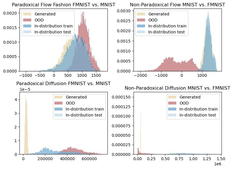
In the paper “A Geometric Explanation of the Likelihood OOD Detection Paradox” (Kamkari, Ross, Cresswell, et al. 2024), the hyperparameters related to the LID estimation are calibrated using the training data an an external model-free LID estimator. Some prior and follow-up work such as LIDL (Tempczyk et al. 2022) and FLIPD (Kamkari, Ross, Hosseinzadeh, et al. 2024) have shown that model-free estimators are not reliable for high-dimensional image data. Thus, instead of calibrating the hyperparamter \tau using a model-free estimator, we pick a subset of in- and out-of-distribution datapoints and visualize an LID curve: a curve for each datapoint indicating their LID estimate for all different values of \tau. Through this, we illustrate how the LID of OOD datapoints when they have a higher likelihood estimate (are paradoxical) is generally lower than the LID of in-distribution datapoints, without the need for any calibration.
Similar to before, we use an appropriate callback to do so and this will log certain artifacts in mlflow:
# fmnist vs. mnist on flows
python scripts/train.py dataset=fmnist +dataset_ood=mnist +experiment=train_flow_greyscale +checkpoint=flow_fmnist +ood=flow_lid_curve
# mnist vs. fmnist on flows
python scripts/train.py dataset=mnist +dataset_ood=fmnist +experiment=train_flow_greyscale +checkpoint=flow_mnist +ood=flow_lid_curve
# fmnist vs. mnist on diffusions
python scripts/train.py dataset=fmnist +dataset_ood=mnist +experiment=train_diffusion_greyscale +checkpoint=diffusion_fmnist +ood=diffusion_lid_curve
# mnist vs. fmnist on diffusions
python scripts/train.py dataset=mnist +dataset_ood=fmnist +experiment=train_diffusion_greyscale +checkpoint=diffusion_mnist +ood=diffusion_lid_curve
Again, each run will create an artifact directory and you can store them in the .env file using the following commands:
dotenv set OOD_LID_CURVE_FLOW_FMNIST <corresponding_artifact_dir>
dotenv set OOD_LID_CURVE_FLOW_MNIST <corresponding_artifact_dir>
dotenv set OOD_LID_CURVE_DIFFUSION_FMNIST <corresponding_artifact_dir>
dotenv set OOD_LID_CURVE_DIFFUSION_MNIST <corresponding_artifact_dir>
Now, by looking at the artifact directories, we will notice that we will have the same structure as before:
lid_curve_generated: This contains the LID curve of the generated data.lid_curve_in_distr_train: This contains the LID curve of the in-distribution data from the training set.lid_curve_in_distr_test: This contains the LID curve of the in-distribution data from the test set.lid_curve_ood: This contains the LID curve of the OOD data.Each of these files will already contain the LID curve png file in trends/trend_epoch=xxx.png. We care about the raw data here, which is inside a csv file trends/trend_epoch=xxx.csv. Here, we will use the csv files of lid_curve_in_distr_test versus the lid_curve_ood and the following code will visualize the LID curves for the in-distribution and OOD data.
%autoreload 2
import dotenv
import matplotlib.pyplot as plt
import pandas as pd
import re
from visualization.pretty import ColorTheme
from visualization.trend import plot_trends
# load the environment variables
dotenv.load_dotenv(override=True)
import os

def visualize_lid_ood_curve(ax, artifact_dir: str, title: str, alpha=0.01, x_label="Sweeping argument", y_label="LID"):
    # find the directory {artifact_dir}/likelihood_generated/metrics=xxx.csv`
    lid_curve_dir = os.path.join(artifact_dir, "lid_curve_in_distr_test", "trends")
    trend_files = [f for f in os.listdir(lid_curve_dir) if re.match(r'trend_epoch=\d+\.csv', f)][0]
    trend_in = pd.read_csv(os.path.join(lid_curve_dir, trend_files), index_col=0).values

    lid_curve_dir = os.path.join(artifact_dir, "lid_curve_ood", "trends")
    trend_files = [f for f in os.listdir(lid_curve_dir) if re.match(r'trend_epoch=\d+\.csv', f)][0]
    trend_ood = pd.read_csv(os.path.join(lid_curve_dir, trend_files), index_col=0).values

    sweeping_args_file = [f for f in os.listdir(lid_curve_dir) if f.startswith("sweeping_range")][0]
    sweeping_args_df = pd.read_csv(os.path.join(lid_curve_dir, sweeping_args_file), index_col=0)

    sweeping_arg = sweeping_args_df.columns[0]
    sweeping_values = sweeping_args_df[sweeping_arg].values
    for i in range(trend_in.shape[0]):
        ax.plot(sweeping_values, trend_in[i], color=ColorTheme.BLUE_FIRST.value, alpha=alpha)
    ax.plot([], [], color=ColorTheme.BLUE_FIRST.value, label="In-distribution")
    for i in range(trend_ood.shape[0]):
        ax.plot(sweeping_values, trend_ood[i], color=ColorTheme.RED_FIRST.value, alpha=alpha)
    ax.plot([], [], color=ColorTheme.RED_FIRST.value, label="OOD")
    ax.set_title(title)
    ax.legend()
    ax.set_xlabel(x_label)
    ax.set_ylabel(y_label)


fig, axs = plt.subplots(2, 2, figsize=(8, 6))

visualize_lid_ood_curve(
    ax=axs[0, 0],
    artifact_dir=os.getenv("OOD_LID_CURVE_FLOW_FMNIST"),
    title="Paradoxical Flow FMNIST vs. MNIST",
    alpha=0.08,
    x_label="$\\log \\tau$",
)
visualize_lid_ood_curve(
    ax=axs[0, 1],
    artifact_dir=os.getenv("OOD_LID_CURVE_FLOW_MNIST"),
    title="Non-Paradoxical Flow MNIST vs. FMNIST",
    alpha=0.08,
    x_label="$\\log \\tau$",
)
visualize_lid_ood_curve(
    ax=axs[1, 0],
    artifact_dir=os.getenv("OOD_LID_CURVE_DIFFUSION_FMNIST"),
    title="Paradoxical Diffusion FMNIST vs. MNIST",
    alpha=0.08,
    x_label="$\\log \\tau$",
)
visualize_lid_ood_curve(
    ax=axs[1, 1],
    artifact_dir=os.getenv("OOD_LID_CURVE_DIFFUSION_MNIST"),
    title="Non-Paradoxical Diffusion MNIST vs. FMNIST",
    alpha=0.08,
    x_label="$\\log \\tau$",
)
# Adjust layout and spacing
plt.tight_layout(pad=1.0)

plt.show()
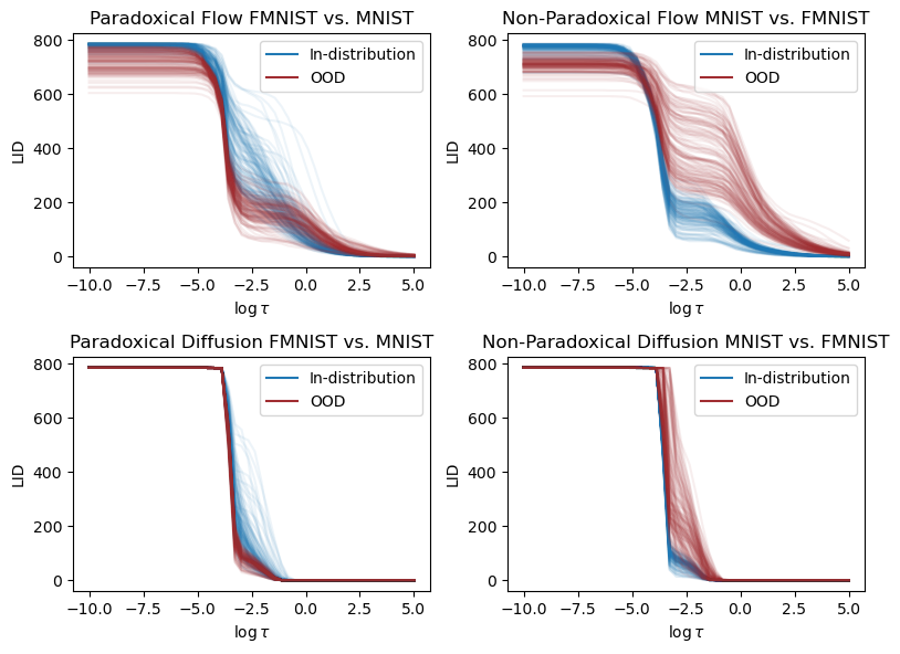
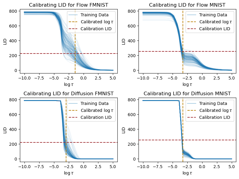
As expected, when \tau \to 0, meaning that \log \tau is very negative, then the LID is estimated as the ambient dimension, and when it is large, it is estimated as zero. Therefore, we have to judiciously pick a \tau value that produces somewhat reasonable estimates. By looking at the curves, it is clear that at certain values of \tau the LID estimate plateaus or shows interesting behaviour. Regardless, looking at the above plots, it is clear that in the paradoxical scenarios (the left half) the LID of in-distribution data is larger than the out-of-distribution counterpart. In fact, for a very small \tau, even on the upper-right, we see that the LID of in-distribution data is larger than the out-of-distribution data which complies with the scatterplot results in (Kamkari, Ross, Cresswell, et al. 2024). Following the paper, let us pick \tau using a calibration procedure that utilizes an external model-free LID estimator. To get access to the calibration LID values, you can run our model-free LID estimator scripts, which under the hood, uses the scikit-dim LPCA estimator. Note that if you run the same script without the alphaFO calibration, it will produce unreasonably small values, such as 8 for FMNIST. This is inline with (Kamkari, Ross, Hosseinzadeh, et al. 2024) where shows that, without tuning, model-free LID estimators are not reliable for high-dimensional image data.
python scripts/model_free_lid.py dataset=fmnist lid_method=lpca +lid_method.estimator.alphaFO=0.001 +experiment=lid_greyscale # will produce ~ 222.48
python scripts/model_free_lid.py dataset=mnist lid_method=lpca +lid_method.estimator.alphaFO=0.001 +experiment=lid_greyscale # will produce ~ 251.62
Note that while these estimates are not reasonable on their own, they give us a baseline to calibrate \tau with. The following piece of code does that logic and visualizes the \tau values that produce the average LID that aligns most with these estimates. By looking at the dashed gold lines, it is easy to see that in the paradoxical scenarios, the \tau value will produce LID estimates on the image above that can separate the in-distribution and out-of-distribution data.
%autoreload 2
import dotenv
import matplotlib.pyplot as plt
import pandas as pd
import re
from visualization.pretty import ColorTheme
from visualization.trend import plot_trends
# load the environment variables
dotenv.load_dotenv(override=True)
import os

def visualize_calibration(
    ax,
    artifact_dir: str,
    title: str,
    calibration_average_lid: float,
    alpha=0.01,
    x_label="Sweeping argument",
    y_label="LID"
):
    # find the directory {artifact_dir}/likelihood_generated/metrics=xxx.csv`
    lid_curve_dir = os.path.join(artifact_dir, "lid_curve_in_distr_train", "trends")
    trend_files = [f for f in os.listdir(lid_curve_dir) if re.match(r'trend_epoch=\d+\.csv', f)][0]
    trend_in = pd.read_csv(os.path.join(lid_curve_dir, trend_files), index_col=0).values

    sweeping_args_file = [f for f in os.listdir(lid_curve_dir) if f.startswith("sweeping_range")][0]
    sweeping_args_df = pd.read_csv(os.path.join(lid_curve_dir, sweeping_args_file), index_col=0)

    sweeping_arg = sweeping_args_df.columns[0]
    sweeping_values = sweeping_args_df[sweeping_arg].values

    best_log_tau = None
    best_avg = None
    for i, val in enumerate(sweeping_values):
        col = trend_in[:, i]
        avg = trend_in[:, i].mean()
        if best_log_tau is None or abs(avg - calibration_average_lid) < abs(best_avg - calibration_average_lid):
            best_log_tau = val
            best_avg = avg

    for i in range(trend_in.shape[0]):
        ax.plot(sweeping_values, trend_in[i], color=ColorTheme.BLUE_FIRST.value, alpha=alpha)
    ax.plot([], [], color=ColorTheme.BLUE_SECOND.value, label="Training Data")
    ax.axvline(x=best_log_tau, color=ColorTheme.PIRATE_GOLD.value, label="Calibrated $\\log \\tau$", linestyle="--")
    ax.axhline(y=calibration_average_lid, color=ColorTheme.RED_FIRST.value, label="Calibration LID", linestyle="--")
    ax.set_title(title)
    ax.legend()
    ax.set_xlabel(x_label)
    ax.set_ylabel(y_label)


fig, axs = plt.subplots(2, 2, figsize=(8, 6))

visualize_calibration(
    ax=axs[0, 0],
    artifact_dir=os.getenv("OOD_LID_CURVE_FLOW_FMNIST"),
    calibration_average_lid=222.48,
    title="Calibrating LID for Flow FMNIST",
    alpha=0.08,
    x_label="$\\log \\tau$",
)
visualize_calibration(
    ax=axs[0, 1],
    artifact_dir=os.getenv("OOD_LID_CURVE_FLOW_MNIST"),
    calibration_average_lid=251.62,
    title="Calibrating LID for Flow MNIST",
    alpha=0.08,
    x_label="$\\log \\tau$",
)
visualize_calibration(
    ax=axs[1, 0],
    artifact_dir=os.getenv("OOD_LID_CURVE_DIFFUSION_FMNIST"),
    calibration_average_lid=222.48,
    title="Calibrating LID for Diffusion FMNIST",
    alpha=0.08,
    x_label="$\\log \\tau$",
)
visualize_calibration(
    ax=axs[1, 1],
    artifact_dir=os.getenv("OOD_LID_CURVE_DIFFUSION_MNIST"),
    calibration_average_lid=251.62,
    title="Calibrating LID for Diffusion MNIST",
    alpha=0.08,
    x_label="$\\log \\tau$",
)
plt.tight_layout(pad=1.0)
plt.show()
We note that the calibration step seems somewhat arbitrary! Indeed, as long as \tau is set such that the in- and out-of-distribution LID estimates are well-separated, it should be good enough for OOD detection. Therefore, while we use this calibration for generating the results in our paper, here we set \tau to a fixed value for simplicity. In the following we fix \tau such that \log \tau = -3. The reason why we fix it to that value is that by looking at the training data, it seems to be a reasonable \tau value where “interesting” things happen in the LID curve for training data.
By fixing the threshold value, we can now run the following command to jointly logging the likelihood and LID values of the in-distribution and OOD data.
# fmnist vs. mnist on flows
python scripts/train.py dataset=fmnist +dataset_ood=mnist +experiment=train_flow_greyscale +checkpoint=flow_fmnist +ood=flow_lid_likelihood +lid_metric.singular_value_threshold=-3
# mnist vs. fmnist on flows
python scripts/train.py dataset=mnist +dataset_ood=fmnist +experiment=train_flow_greyscale +checkpoint=flow_mnist +ood=flow_lid_likelihood +lid_metric.singular_value_threshold=-3
# fmnist vs. mnist on diffusions
python scripts/train.py dataset=fmnist +dataset_ood=mnist +experiment=train_diffusion_greyscale +checkpoint=diffusion_fmnist +ood=diffusion_lid_likelihood +lid_metric.singular_value_threshold=-3
# mnist vs. fmnist on diffusions
python scripts/train.py dataset=mnist +dataset_ood=fmnist +experiment=train_diffusion_greyscale +checkpoint=diffusion_mnist +ood=diffusion_lid_likelihood +lid_metric.singular_value_threshold=-3
Again, each run will create an artifact directory and you can store them in the .env file using the following commands:
dotenv set OOD_LID_LIKELIHOOD_FLOW_FMNIST_1 <corresponding_artifact_dir>
dotenv set OOD_LID_LIKELIHOOD_FLOW_MNIST_1 <corresponding_artifact_dir>
dotenv set OOD_LID_LIKELIHOOD_DIFFUSION_FMNIST_1 <corresponding_artifact_dir>
dotenv set OOD_LID_LIKELIHOOD_DIFFUSION_MNIST_1 <corresponding_artifact_dir>%autoreload 2
import dotenv
import matplotlib.pyplot as plt
import pandas as pd
from visualization.pretty import ColorTheme
# load the environment variables
dotenv.load_dotenv(override=True)
import os
def visualize_scatterplot(
ax,
artifact_dir: str,
title: str,
alpha=0.01,
):
# find the directory {artifact_dir}/likelihood_generated/metrics=xxx.csv`
likelihood_dir = os.path.join(artifact_dir, "lid_likelihood_generated")
metrics_dir = [f for f in os.listdir(likelihood_dir) if f.startswith("metrics")][0]
metrics_dir = os.path.join(likelihood_dir, metrics_dir)
likelihood_generated = pd.read_csv(metrics_dir)['likelihood']
lid_generated = pd.read_csv(metrics_dir)['JacobianThresholdLID']
likelihood_dir = os.path.join(artifact_dir, "lid_likelihood_ood")
metrics_dir = [f for f in os.listdir(likelihood_dir) if f.startswith("metrics")][0]
metrics_dir = os.path.join(likelihood_dir, metrics_dir)
likelihood_ood = pd.read_csv(metrics_dir)['likelihood']
lid_ood = pd.read_csv(metrics_dir)['JacobianThresholdLID']
likelihood_dir = os.path.join(artifact_dir, "lid_likelihood_in_distr_train")
metrics_dir = [f for f in os.listdir(likelihood_dir) if f.startswith("metrics")][0]
metrics_dir = os.path.join(likelihood_dir, metrics_dir)
likelihood_in_distr_train = pd.read_csv(metrics_dir)['likelihood']
lid_in_distr_train = pd.read_csv(metrics_dir)['JacobianThresholdLID']
likelihood_dir = os.path.join(artifact_dir, "lid_likelihood_in_distr_test")
metrics_dir = [f for f in os.listdir(likelihood_dir) if f.startswith("metrics")][0]
metrics_dir = os.path.join(likelihood_dir, metrics_dir)
likelihood_in_distr_test = pd.read_csv(metrics_dir)['likelihood']
lid_in_distr_test = pd.read_csv(metrics_dir)['JacobianThresholdLID']
# plot an overlapping histogram
ax.scatter(likelihood_generated, lid_generated, alpha=alpha, label="Generated", color=ColorTheme.GOLD.value)
ax.scatter(likelihood_ood, lid_ood, alpha=alpha, label="OOD", color=ColorTheme.RED_FIRST.value)
ax.scatter(likelihood_in_distr_train, lid_in_distr_train, alpha=alpha, label="In-distribution train", color=ColorTheme.BLUE_FIRST.value)
ax.scatter(likelihood_in_distr_test, lid_in_distr_test, alpha=alpha, label="In-distribution test", color=ColorTheme.BLUE_SECOND.value)
ax.set_xlabel("Log Likelihood")
ax.set_ylabel("LID(.;$\\tau$)")
ax.set_title(title)
ax.legend()
return {
"generated": (likelihood_generated, lid_generated),
"ood": (likelihood_ood, lid_ood),
"in_distr_train": (likelihood_in_distr_train, lid_in_distr_train),
"in_distr_test": (likelihood_in_distr_test, lid_in_distr_test),
}
fig, axs = plt.subplots(2, 2, figsize=(8, 6))
lid_likelihood_flow_fmnist_1 = visualize_scatterplot(
ax=axs[0, 0],
artifact_dir=os.getenv("OOD_LID_LIKELIHOOD_FLOW_FMNIST_1"),
title="Scatterplot on Flow FMNIST ($\\log \\tau=-3$)",
alpha=0.6,
)
lid_likelihood_flow_mnist_1 = visualize_scatterplot(
ax=axs[0, 1],
artifact_dir=os.getenv("OOD_LID_LIKELIHOOD_FLOW_MNIST_1"),
title="Scatterplot on Flow MNIST ($\\log \\tau=-3$)",
alpha=0.6,
)
lid_likelihood_diffusion_fmnist_1 = visualize_scatterplot(
ax=axs[1, 0],
artifact_dir=os.getenv("OOD_LID_LIKELIHOOD_DIFFUSION_FMNIST_1"),
title="Scatterplot on Diffusion FMNIST ($\\log \\tau=-3$)",
alpha=0.6,
)
lid_likelihood_diffusion_mnist_1 = visualize_scatterplot(
ax=axs[1, 1],
artifact_dir=os.getenv("OOD_LID_LIKELIHOOD_DIFFUSION_MNIST_1"),
title="Scatterplot on Diffusion FMNIST ($\\log \\tau=-3$)",
alpha=0.6,
)
plt.tight_layout(pad=1.0)
plt.show()
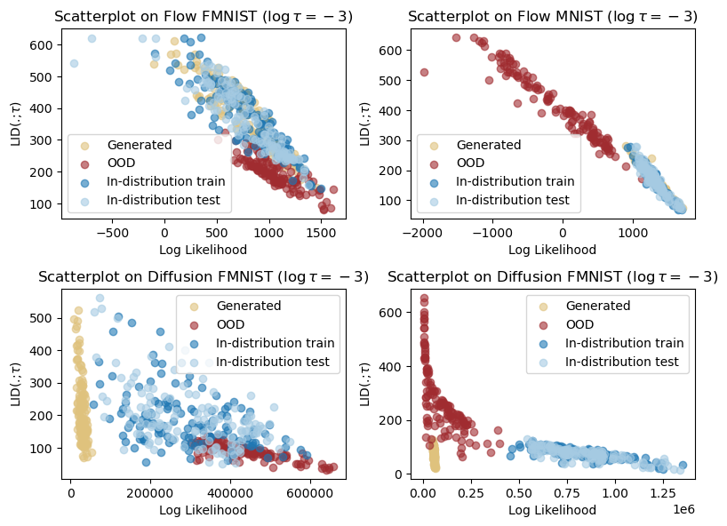
We will also try out another \tau value below to show that LID is not always inversely related to likelihood.
# fmnist vs. mnist on flows
python scripts/train.py dataset=fmnist +dataset_ood=mnist +experiment=train_flow_greyscale +checkpoint=flow_fmnist +ood=flow_lid_likelihood +lid_metric.singular_value_threshold=-5
# mnist vs. fmnist on flows
python scripts/train.py dataset=mnist +dataset_ood=fmnist +experiment=train_flow_greyscale +checkpoint=flow_mnist +ood=flow_lid_likelihood +lid_metric.singular_value_threshold=-5
# save the artifact directories
dotenv set OOD_LID_LIKELIHOOD_FLOW_FMNIST_2 <corresponding_artifact_dir>
dotenv set OOD_LID_LIKELIHOOD_FLOW_MNIST_2 <corresponding_artifact_dir>fig, axs = plt.subplots(1, 2, figsize=(8, 3))
lid_likelihood_flow_fmnist_2 = visualize_scatterplot(
ax=axs[0],
artifact_dir=os.getenv("OOD_LID_LIKELIHOOD_FLOW_FMNIST_2"),
title="Scatterplot on Flow FMNIST ($\\log \\tau=-5$)",
alpha=0.6,
)
lid_likelihood_flow_mnist_2 = visualize_scatterplot(
ax=axs[1],
artifact_dir=os.getenv("OOD_LID_LIKELIHOOD_FLOW_MNIST_2"),
title="Scatterplot on Flow MNIST ($\\log \\tau=-5$)",
alpha=0.6,
)
plt.tight_layout(pad=1.0)
# The hyperparameter setting is not good for diffusion models
plt.show()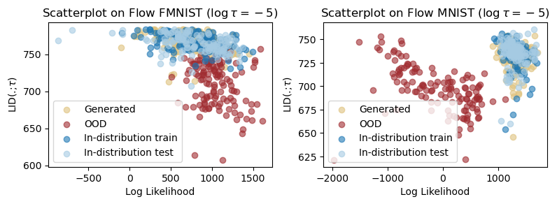
We finally show how to evaluate the OOD detection results. To do so, we will use the dual threshold algorithm, where a datapoint is in-distribution if it has both high likelihood and high LID values, which translates to larger probability mass around the datapoint. We have recorded the LID and likelihood estimates of the above scatterplots. Run the following script to evaluate the results:
from metrics.ood.roc_analysis import get_roc_graph, get_pareto_frontier, get_auc


def get_aucs(results_dict):
    ret = {}
    likelihood_generated, lid_generated = results_dict["generated"]
    likelihood_in_distr, lid_in_distr = results_dict["in_distr_test"]
    likelihood_ood, lid_ood = results_dict["ood"]

    roc_x, roc_y = get_roc_graph(
        pos_x=likelihood_in_distr,
        neg_x=likelihood_ood,
        verbose=0,
    )
    pareto_x, pareto_y = get_pareto_frontier(
        roc_x, roc_y,
    )
    ret["Single Threshold (In-Distr vs. OOD)"] = get_auc(pareto_x, pareto_y)
    roc_x, roc_y = get_roc_graph(
        pos_x=likelihood_generated,
        neg_x=likelihood_ood,
        verbose=0,
    )
    pareto_x, pareto_y = get_pareto_frontier(
        roc_x, roc_y,
    )
    ret["Single Threshold (Generated vs. OOD)"] = get_auc(pareto_x, pareto_y)

    roc_x, roc_y = get_roc_graph(
        pos_x=likelihood_in_distr,
        pos_y=lid_in_distr,
        neg_x=likelihood_ood,
        neg_y=lid_ood,
        verbose=0,
    )
    pareto_x, pareto_y = get_pareto_frontier(
        roc_x, roc_y,
    )
    ret["Dual Threshold (In-Distr vs. OOD)"] = get_auc(pareto_x, pareto_y)
    roc_x, roc_y = get_roc_graph(
        pos_x=likelihood_generated,
        pos_y=lid_generated,
        neg_x=likelihood_ood,
        neg_y=lid_ood,
        verbose=0,
    )
    pareto_x, pareto_y = get_pareto_frontier(
        roc_x, roc_y,
    )
    ret["Dual Threshold (Generated vs. OOD)"] = get_auc(pareto_x, pareto_y)
    return ret

rows = [
    "Single Threshold (In-Distr vs. OOD)",
    "Dual Threshold (In-Distr vs. OOD)",
    "Single Threshold (Generated vs. OOD)",
    "Dual Threshold (Generated vs. OOD)",
]
columns = [
    ("Normalizing flow [FMNIST vs. MNIST]", lid_likelihood_flow_fmnist_1),
    ("Normalizing flow [MNIST vs. FMNIST]", lid_likelihood_flow_mnist_1),
    ("Diffusion [FMNIST vs. MNIST]", lid_likelihood_diffusion_fmnist_1),
    ("Diffusion [MNIST vs. FMNIST]", lid_likelihood_diffusion_mnist_1),
]
df = pd.DataFrame(index=rows, columns=[key for key, _ in columns])
# create a
for key, auc_dict in columns:
    for key2, value in get_aucs(auc_dict).items():
        df.loc[key2, key] = value
df| Normalizing flow [FMNIST vs. MNIST] | Normalizing flow [MNIST vs. FMNIST] | Diffusion [FMNIST vs. MNIST] | Diffusion [MNIST vs. FMNIST] | |
|---|---|---|---|---|
| Single Threshold (In-Distr vs. OOD) | 0.291138 | 0.999207 | 0.197205 | 1.0 |
| Dual Threshold (In-Distr vs. OOD) | 0.949707 | 0.999207 | 0.90802 | 1.0 |
| Single Threshold (Generated vs. OOD) | 0.228699 | 0.999268 | 0.0 | 0.430664 |
| Dual Threshold (Generated vs. OOD) | 0.951355 | 0.999268 | 0.948669 | 0.436157 |
As you can see, the dual threshold algorithm is a simple yet effective way to detect OOD data. We also note that with this hyperparameter setup the Diffusion generated vs. OOD does not give us a good separation, however, by judiciously picking the \tau value, we can get a good separation on that task too.
Throughout this notebook, we used FMNIST and MNIST as our illustrative datasets. However, you can easily extend this to other datasets by following the same steps above and would arrive at similar results. You can use our dataset to train on other image datasets as well, and we support them through our HuggingFace integration, we have already included the CIFAR10 and SVHN datasets in our codebase. Finally, while most of these observations have been made on image datasets, we also support training diffusion models and normalizing flows for tabular datasets in our codebase. However, the likelihood paradox is not as pronounced in tabular datasets as it is in image datasets.